| Passenger Class | Frequency |
|---|---|
| First | 323 |
| Second | 277 |
| Third | 709 |
| Total | 1,309 |
2 Looking at Distributions
The distribution of a variable refers to how the different values of that variable are spread out across observations. This distribution gives us a sense of what the most common values are for a given variable and how much these values vary. It can also alert us to unusual patterns in the data. Intuitively, we think about distributions in our personal life any time we think about how we “measure up” relative to everyone else on something (e.g. income, number of social media followers, GRE scores, etc.). We want to know where we “fall” in the distribution of one of these variables.
In this chapter we will focus on two ways to gain better insight into the distribution of a variable:
- Graph it. Visualizing a distribution with a good figure is often the first step in trying to understand it.
- Measure it. For quantitative variables, we can move beyond a visual display to calculate summary statistics that provide more precise information about the distribution including its center and spread.
For this chapter, we are only examining the distribution of a single variable. We sometimes refer to this form of analysis and the statistics we calculate from it as univariate, which is a fancy way to say “one variable.” Importantly, univariate analysis of a single variable does not tell us anything about the association of that variable with other variables.
Slides for this chapter can be found here.
Graphing Distributions
One of the best ways to understand the distribution of a variable is to visualize that distribution with a graph. Importantly, the technique we use to graph the distribution will depend on whether we have a categorical or a quantitative variable. For categorical variables, we will use a barplot, while for quantitative variables, we will use a histogram.
Know your variable type!
Remember that categorical and quantitative variables require different kinds of graphs. Knowing which kind of variable you have is the first step to making the right kind of graph!
Graphing the distribution of a categorical variable
Calculating the frequency
In order to graph the distribution of a categorical variable, we first need to calculate its frequency. The frequency is just the number of observations that fall into a given category of a categorical variable. We could, for example, count up the number of passengers who were in the various passenger classes on the Titanic. Doing so would give us the frequencies shown in Table 2.1 below:
The Titanic contained 323 first class passengers, 277 second class passengers, and 709 third class passengers. Adding those numbers up gives us 1,309 total passengers.
We can also calculate these numbers in R using the table command:
table(titanic$pclass)
 First Second  Third
   323    277    709
Commands in R
table is an example of a command (or function) in R. R comes with many built-in functions and more can be added from additional packages/libraries. You can even create your own! These commands will be the workhorse for us as they can do all kinds of calculations.
Command names are always followed by and opening and closing parenthesis and inside of those parenthesis you can feed in input called arguments. In this case, we just need one argument which is the variable for which we want the frequencies. Remember that we have to specify this with our dataset_name$variable_name syntax. One translation of this command in English would be “create a table of the passenger class variable from the Titanic dataset.”
Although this command only had one argument, many commands can have multiple arguments. When a command has more than one argument, we separate them inside the parenthesis with commas. We will see some examples of multiple arguments commands below when we get to ggplot commands.
Frequency, proportion, and percent
The frequency we just calculated is called the absolute frequency because it counts the raw number of observations. However such raw numbers are often not very helpful because they will vary by the overall number of observations. If I told you out of context that there were 323 first class passengers on the Titanic, would you think that is a large or small number? Most likely, you would want to know how many total passengers there were on the Titanic tp get a sense of the share of first class passengers out of the total number of passengers..
Instead of relying on the absolute frequency, we generally calculate the proportion of observations that fall within each category. These proportions are sometimes also called the relative frequency. We can calculate the proportion by simply dividing our absolute frequency by the total number of observations as shown in Table 2.2.
| Passenger Class | Frequency | Proportion | |
|---|---|---|---|
| First | 323 | 0.247 | (323/1309) |
| Second | 277 | 0.212 | (277/1309) |
| Third | 709 | 0.542 | (709/1309) |
| Total | 1,309 | 1 |
We can confirm that our calculations are correct by noting that the proportions add up to 1 (plus or minus a bit of rounding error).
R provides a nice shorthand function titled prop.table to conduct this operation. The prop.table command should be run on the output from a table command.
prop.table(table(titanic$pclass))
    First    Second     Third
0.2467532 0.2116119 0.5416348
Wrapping Commands vs. Saving Output in R
Note that I have “wrapped” one command (table) inside of another command (prop.table). In essence, the output of the table command became the input of the prop.table command. R is fine with this kind of code and we can often use this wrapping feature to take care of multiple operations in one line of code.
Alternatively, I could have “saved” the output of my table command and then fed that saved output into the prop.table command. That code would look something like:
tab <- table(titanic$pclass)
prop.table(tab)
The <- is an assignment operator. It tells R that instead of printing the output of table to the screen, it should instead save that output to a new object. I call that object “tab” but I could have called it anything I want. I then feed that tab object into prop.table on the second line.
The reason we often prefer to wrap commands as I did above is that it reduces the lines of code and also avoids the creation of temporary data artifacts like the tab object. However, there may be some cases where you want to save output to an object, so its good to know how to do this.
We often convert proportions to percents which are more familiar to most people. To convert a proportion to a percent, just multiply by 100 as shown in Table 2.3.
| Passenger Class | Frequency | Proportion | Percent | ||
|---|---|---|---|---|---|
| First | 323 | 0.247 | (323/1309) | 24.7% | (100*0.247) |
| Second | 277 | 0.212 | (277/1309) | 21.2% | (100*0.212) |
| Third | 709 | 0.542 | (709/1309) | 54.2% | (100*0.542) |
| Total | 1,309 | 1 | 100 |
24.7% of passengers were first class, 21.2% of passengers were second class, and 54.2% of passengers were third class. Just over half of passengers were third class and the remaining passengers were fairly evenly split between first and second class.
Make a barplot
Now that we have the proportions/percents, we can visualize the distribution with a barplot in which vertical or horizontal bars give the proportion or percent. To build this barplot, we need to use ggplot. The ggplot syntax is a little different than most of the other R syntax we will use, but its very important because we will use ggplot to build all of our figures. With ggplot, we add several commands together with the + sign to create our overall plot. Each command adds a “layer” to our plot. To help you understand how ggplot works, I have annotated the code to produce Figure 2.1 below to show you what each element is doing.
1ggplot(titanic, aes(x=pclass, y=after_stat(prop), group=1))+
2  geom_bar()+
3  labs(x="passenger class", y="percent")+
4  scale_y_continuous(labels=scales::percent)+
5  coord_flip()+
6 theme_bw()- 1
-
The first command is always the
ggplotcommand itself which defines the dataset we will use (in this case,titanic) and the “aesthetics” that are listed in theaesargument. In this case, I defined an x (horizontal) variable as thepclassvariable itself and the y (vertical) variable as a proportion (which in ggplot-speak isafter_stat(prop)). Thegroup=1argument is a trick for barplots that ensures the proportions are calculated based on the total sample. I can then continue to add other elements to the plot by connecting them with a+. - 2
-
The
geom_baris an example of ageom_command, which tells ggplot what actual shapes to plot on the canvas - in this case, bars. At this point, I have a functional barplot, but I am going to connect other arguments with the+sign to make the figure look nicer. - 3
-
The
labscommand allows us to specify nice looking labels for the final figure. Here I use it to specify nice labels for the x and y axis. Always label your figure nicely! - 4
-
The
scale_commands are not necessary but can be used when you want finer control over how the scale of one of your aesthetics (e.g. x, y, fill, color) is displayed. In this case, I am using it to make the y-axis tickmark labels display as percentages. - 5
-
The
coord_flipcommand will flip the x and y axis. This is useful when you have long labels on a categorical variable that will operlap on the x-axis. - 6
-
The
theme_bw(bw for black and white) sets an overall theme for the figure. I like the clean look oftheme_bwand use it for most figures in this book.
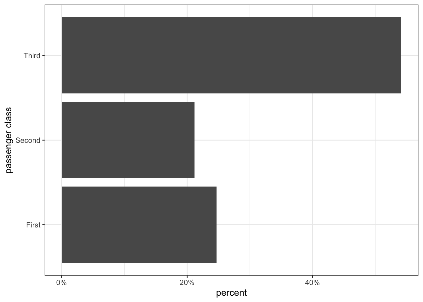
Figure 2.1 shows a barplot for the distribution of passengers on the Titanic. We can clearly see that third class is the largest passenger class with slightly more than 50% of all passengers. We also can easily determine visually that third class passengers are more than twice as common as either of the other two categories, simply by comparing the height of the bars. We can also see that slightly more passengers were in first class than second class simply by comparing the heights of those two bars.
Don’t forget the +!
To construct a figure with ggplot2, you string together multiple commands with the “+” sign. A very common mistake is to miss a “+” which will break the chain and end your plot. So, if your plot is not looking right, one of the first things to check is whether you missed a “+” somewhere.
You will note that I place each separate command that is part of the ggplot on a separate line and indent subsequent commands after the ggplot command. This helps me to visually tell which bits of code are part of the ggplot. RStudio will do this indenting for you by default and you can also force it to do a line-by-line re-indenting with the Control+I hotkey (or Command+I in Mac). Re-indenting your lines provides an easy check on this problem because a missing “+” will mean that subsequent lines will not be indented.
Never use piecharts!
You may have seen the distributions I am showing here also displayed using a piechart like Figure 2.2 below.

Many people feel that piecharts have an aesthetic appeal but they are actually very poor at conveying information relative to barplots. Why? In order to judge the relative size of the slices on a piechart, your eye has to make judgments in two dimensions and with an unusual pie-shaped slice (\(\pi*r^2\) anyone?). As a result, it can often be difficult to decide which slice is bigger and to properly evaluate the relative sizes of each of the slices. In this case, for example, the relative size of first and second class are quite close and it is not immediately obvious which category is larger. Because barplots only work in one dimension, we can much more clearly gauge the relative size of each bar in Figure 2.1 which shows that first class was larger than second class by about 3-4%.
Graphing the distribution of a quantitative variable
Barplots won’t work for quantitative variables because quantitative variables don’t have categories. However, we can do something quite similar with the histogram.
One way to think about the histogram is that we are imposing a set of categories on a quantitative variable by breaking our quantitative variable into a set of equally wide intervals that we call bins. The most important decision with a quantitative variable is how wide to make these bins. As an example, lets calculate 10-year bins for the age variable in the politics dataset. Because the youngest people in this dataset are 18 years old, I could start my first bin at age 18 and go to age 27. However, that will give me somewhat non-intuitive bins for most people (e.g. 18-27, 28-37, etc.). Instead, I will start my first bin at 15-24, so the bins are “cut” at the mid-decade point for each age group (e.g. 15-24, 25-34, 35-44, etc.). Then, I count the number of observations that fall into each age bin as shown in Table 2.4.
| Age bin | Frequency |
|---|---|
| 15-24 | 339 |
| 25-34 | 725 |
| 35-44 | 672 |
| 45-54 | 708 |
| 55-64 | 828 |
| 65-74 | 629 |
| 75-84 | 254 |
| 15-94 | 82 |
Now that I have the frequencies for each bin, I can plot the histogram. The histogram looks much like a barplot except for two important differences. First, on the x-axis we have a numeric scale for the quantitative variable rather than categories. Second, we don’t put any space between our bars.
The annotated code below shows you how to create the histogram in Figure 2.3 using ggplot.
1ggplot(politics, aes(x=age))+
2  geom_histogram(binwidth=10, col="black", fill="grey",
                 closed="left")+
3  labs(x="age")+
theme_bw()- 1
- For the histogram case, we only need to specify an x aesthetic, defined by whichever variable we want to get a histogram for.
- 2
-
The
geom_histogramcommand will do most of the work of creating the histogram. Thebinwidthargument is the critical argument here because it defines how large each bin is. You will need to adjust this number as necessary depending on your case. Thecolandfilldefine border and fill colors, respectively for the bars. You can specify specific colors like this for mostgeom_elements. To see a list of built-in color choices in R, typecolors()in the console. - 3
-
Always remember to use
labsto nicely label your result.
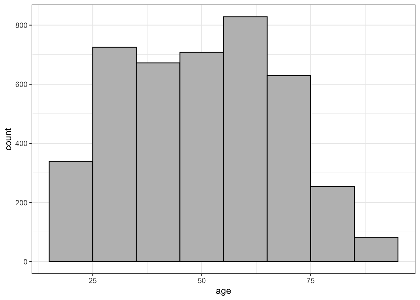
Looking at Figure 2.3, I see the peak in the distribution in the 55-64 group (the baby boomers) with a plateau to the left at younger ages before dropping off for the youngest age group, due to the fact that this youngest age group is only a partial age group (e.g. I have no 15-17 year olds). To the right, the frequency drops off much faster, due to smaller cohorts and old age mortality. I can also sort of see a smaller peak in the 25-34 range which happens to be the children of the baby boomers.
What would this histogram look like if I had used 5-year bin widths instead of 10-year bins? Lets try it:
ggplot(politics, aes(x=age))+
  geom_histogram(binwidth=5, col="black", fill="grey",
                 closed="left")+
  labs(x="age")+
  theme_bw()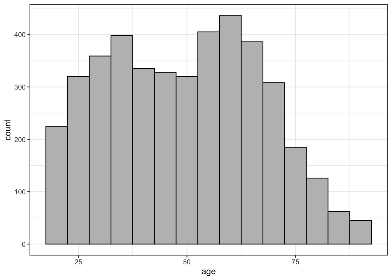
As Figure 2.4 shows, I get more or less the same overall impression but a more fine-grained view. I can more easily pick out the two distinct “humps” in the distribution that correspond to the baby boomers and their children. Sometimes adjusting bin width can reveal or hide important trends and sometimes it can just make it more difficult to visualize the distribution. As an exercise, you can play around with the interactive example below.
What kinds of things should you be looking for in your histogram? There are four general things to be on the lookout for when you examine a histogram.
Center
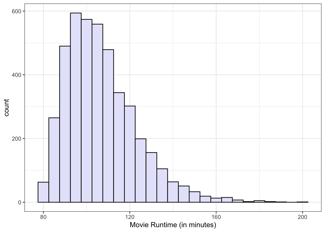
Where is the center of the distribution? Loosely we can think of the center as the peak in the data, although we will develop some more technical terms for center below. Some distributions might have more than one distinct peak. When a distribution has one peak, we call it a unimodal distribution. Figure 2.5 (a) shows a clear unimodal distribution for the runtime of movies. We can clearly see that the peak is somewhere between 90 and 100 minutes.

When a distribution has two distinct peaks, we call it a bimodal distribution. Figure 2.5 (b) shows that the distribution of violent crime rates across states is bimodal. The first peak is around 2200-2500 crimes per 100,000 and the second is around 3500 crimes per 100,000. This suggests that there are two distinctive clusters of states: in the first cluster are states with a moderate crime rate and in the second cluster, states with high crime rate states. You can probably guess what we call a distribution with three peaks (and so on), but its fairly rare to see more than two distinct peaks in a distribution.
Shape
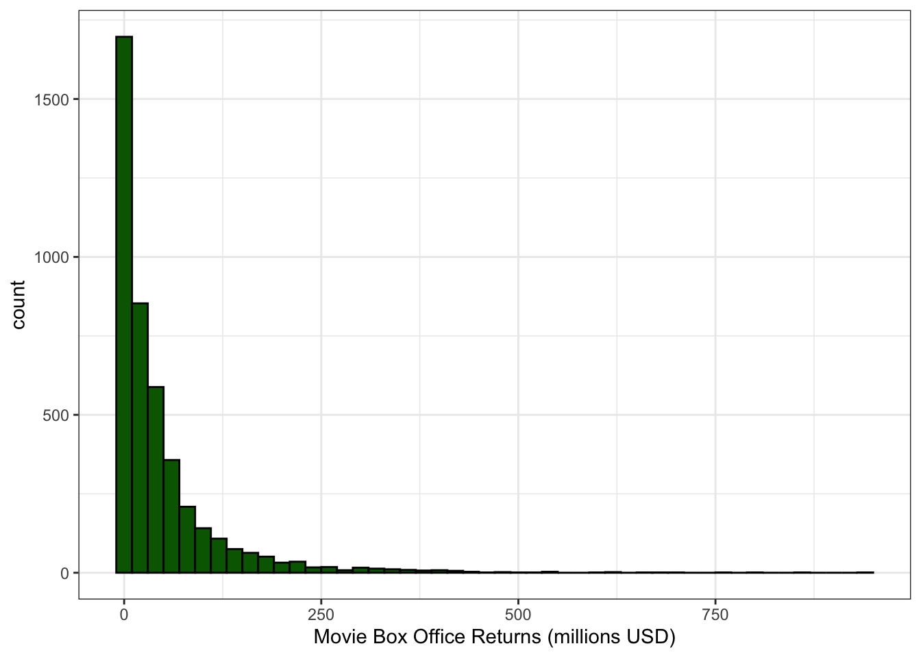
Is the shape symmetric or is one of the tails longer than the other? When the long tail is on the right, we refer to this distribution as right skewed. When the long tail is on the left, we refer to the distribution as left skewed. Figure 2.6 (a) and Figure 2.6 (b) show examples of roughly symmetric and heavily right-skewed distributions, respectively, from the movies dataset. The Metacritic score that movies receive (from 0-100) is roughly symmetric with about equal numbers of movies above and below the peak. Box office returns on the other hand are heavily right-skewed. Most movies make less than $100 million at the box office but there are a few blockbusters that rake in far more money. Right-skewness to some degree or another is common in social science data, partially because many variables can’t logically have values below zero and thus the left tail of the distribution is truncated. Left-skewed distributions are rare. In fact, they are so rare that I don’t really have a very good example to show you from our datasets.

Spread
How spread out are the values around the center? Do they cluster tightly around the center or are they spread out more widely? Typically this is a question that can only be asked in relative terms. We can only say that the spread of a distribution is larger or smaller than some comparable distribution. We might be interested for example in the spread of the income distribution in the US compared to Sweden, because this spread is one measure of income inequality.
Figure 2.7 compares the distribution of movie runtime for comedy and sci-fi/fantasy movies. The figure clearly shows that the spread of movie runtime is much greater for sci-fi/fantasy movies. Comedy movies are all tightly clustered between 90 and 120 minutes while longer movies are more common for the sci-fi/fantasy genre, leading to a longer right tail and a correspondingly higher spread.

Outliers
Are there extreme values which fall outside the range of the rest of the data? We want to pay attention to these values because they may have a strong influence on the statistics that we will calculate to summarize a distribution. They might also influence some of the measures of association that we will learn later. Finally, extreme outliers may help identify data coding errors.
In Figure 2.5 (b) above, we can see that Washington DC is a clear outlier in terms of the violent crime rate. Washington DC’s crime rate is such an outlier relative to the other states that we will pay attention to it throughout this term as we conduct our analysis. Figure 2.7 above shows that Peter Jackson’s Return of the King was an outlier for the runtime of sci-fi/fantasy movies, although it doesn’t seem quite as extreme as for the case of Washington DC.
In large datasets, it can sometimes be very difficult to detect a single outlier on a histogram because the height of its bar will be so small. You probably wouldn’t even notice the Return of the King outlier in the movies dataset if I hadn’t labeled it. Later in this chapter, we will learn another graphical technique called the boxplot that can be more useful for detecting outliers in a quantitative variable.
Adding a pop of color
You will notice that I added some color to many of the histograms in this section. How do you do that? As the code for Figure 2.4 above showed, you can specify a fill and border color for the bars in geom_histogram with the col and fill arguments respectively. So for example, I could have done the histogram of age above with some brighter color choices:
ggplot(politics, aes(x=age))+
  geom_histogram(binwidth=5, col="green", fill="yellow",
                 closed="left")+
  labs(x="age")+
  theme_bw()
You might be wondering how many color names R knows. You can quickly find out by typing colors() into the R console. This will give you a full list of 657 color names that R knows. For example, lets see what the figure looks like with a fill color of “wheat” and border color of “steelblue.”
ggplot(politics, aes(x=age))+
  geom_histogram(binwidth=5, col="steelblue", fill="wheat",
                 closed="left")+
  labs(x="age")+
  theme_bw()
If these color options are not enough for you, you can also specify a color using a hex code made up of six alphanumeric characters. You can find many color picker apps online that will give you a specific hex code. For example, lets say you wanted to use hex codes for the Oregon Duck colors:
ggplot(politics, aes(x=age))+
  geom_histogram(binwidth=5, col="#FEE123",fill="#154733",
                 closed="left")+
  labs(x="age")+
  theme_bw()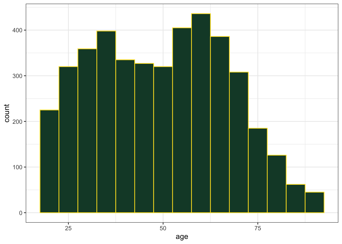
You can color many of the geoms we will use in ggplot the same way, although whether you use fill or col or both will depend on the geom. For example, we can also color barplots in the same way as histograms:
ggplot(titanic, aes(x=pclass, y=after_stat(prop), group=1))+
  geom_bar(fill="plum", col="dodgerblue")+
  labs(x="passenger class", y="percent")+
  scale_y_continuous(labels=scales::percent)+
  coord_flip()+
theme_bw() 
We will also learn later that we can use color as an aesthetic in the aes command. In that case, color will be used to tell us some important information and instead of choosing raw colors, we can instead choose a color palette. Look for more information on this approach in the next chapter.
Measuring the Center of a Distribution
In the previous section, we just looked at a distribution to try and gauge its center. But what do we really mean by the term “center?” We often think about the center intuitively as representing the “typical” or “average” value of a given variable. However, we can define this idea of “average” in multiple ways. In this section, we will move from a basic visual sense of center to more precise statistical measures of center that can be calculated for quantitative variables. Specifically, we will learn how to measure the mean, median, and mode.
The mean
The mean is the measure most frequently referred to as the “average” although that term could apply to the median and mode as well. The mean is the balancing point of a distribution. Imagine trying to balance a distribution on your finger like a basketball. Where along the distribution would you place your finger to achieve balance? This point is the mean. It is equivalent to the concept of “center of mass” from physics.
The calculation of the mean is straightforward:
- Sum up all the values of your variable across all observations.
- Divide this sum by the number of observations.
As a workable example, lets take a sub-sample of our movie data with a small number of observations. I am going to select all nine “pure” romance movies produced in 2017 (not including romantic comedies which are coded as comedies rather than romances on the genre variable). Table 2.5 displays these movies along with their Metacritic score.
| Title | Metacritic Score |
|---|---|
| Call Me by Your Name | 93 |
| Disobedience | 74 |
| Everything, Everything | 52 |
| Fifty Shades Darker | 33 |
| Kings | 34 |
| My Cousin Rachel | 63 |
| Phantom Thread | 90 |
| Tulip Fever | 38 |
| Wonder Wheel | 45 |
| Sum | 522 |
In the very last row, I show the sum of the Metacritic score which simply sums up the Metacritic score of each movie. With this sum, I am already halfway to calculating the mean! To finish the calculation, I divide this sum (522) by the number of movies (9).
\[\frac{522}{9}=58\]
The mean Metacritic score for romantic movies in 2017 was 58.
Lets use R to calculate mean Metacritic score across all movies. You could use the sum command (self-explanatory) and the nrow command, which will give you the number of observations, to calculate the mean:
sum(movies$metascore)/nrow(movies)[1] 52.74971Alternatively, R already has a command called mean:
mean(movies$metascore)[1] 52.74971We can see that the mean Metacritic score of romantic movies in 2017 (58) was slightly higher the mean for all the movies in our dataset (52.7), but not by much.
Learning equation symbols
We won’t focus too much on formulas in this course, but it is helpful to know some basics of the way mathematical formulas are represented in statistics.
Mathematically, we often represent variables with lower-case roman letters like \(x\) or \(y\). Then we can talk abstractly about “some variable \(x\)” rather than referencing a specific variable. If we want to specify a particular observation of \(x\), we use a subscript number. So \(x_1\) is the value of the first observation of \(x\) in our data and \(x_{25}\) is the value of the 25th observation of \(x\) in our data. We use the letter \(n\) to signify the number of observations so \(x_n\) is always the last observation of \(x\) in our data.
We could use this symbology to describe summing up all the values of \(x\) and dividing by \(n\):
\[\frac{x_1+x_2+x_3+\ldots+x_n}{n}\]
This approach works but can be quite tedious. You can see that I already tired of writing out each value of \(x\) and just used \(\ldots\) to convey the general point. To avoid this, we often use a summation sign to indicate the summing up of all the values of a variable:
\[\sum_{i=1}^n x_i=x_1+x_2+x_3+\ldots+x_n\]
In English, this formula just means “sum up all the values of \(x\), starting at \(x_1\) and ending at \(x_n\).” That gives us our sum, which we just need to divide by the number of observations, \(n\), to get the mean:
\[\bar{x}=\frac{\sum_{i=1}^n x_i}{n}\]
You will notice that I describe this mean using the symbol \(\bar{x}\). This symbol is often called “x-bar” and is the standard way to describe the mean of some variable \(x\). Note that if we had two variables \(x\) and \(y\), then we would have \(\bar{x}\) (x-bar) and \(\bar{y}\) (y-bar) to represent the mean of each variable.
The median
The median is almost as widely used as the mean as a measure of center, for reasons I will discuss below. The median is the midpoint of the distribution. It is the point at which 50% of observations have lower values and 50% of the observations have higher values.
In order to calculate the median, we need to first order our observations from lowest to highest. As an example, in Table 2.6, I take the 2017 romantic movie data from Table 2.5 and re-order it from highest Metacritic score to lowest.
| Title | Metacritic Score | Order |
|---|---|---|
| Call Me by Your Name | 93 | 1 |
| Phantom Thread | 90 | 2 |
| Disobedience | 74 | 3 |
| My Cousin Rachel | 63 | 4 |
| Everything, Everything | 52 | 5 |
| Wonder Wheel | 45 | 6 |
| Tulip Fever | 38 | 7 |
| Kings | 34 | 8 |
| Fifty Shades Darker | 33 | 9 |
To find the median, we have to find the observation right in the middle. When we have an odd number of observations, finding the exact middle is easy. In this case, the fifth observation is the exact middle because it has four observations lower than it and four observations higher than it. So the median Metacritic score for romantic movies in 2017 was 52.
What if you have an even number of observations? Finding the median is slightly more tricky in this case because you have no single observation that is exactly in the middle. Instead, you find the two observations that are closest to the middle and calculate their mean (sum them up and divide by two). For example, if we had ten observations, we would take the mean of the fifth and sixth observations to calculate the median.
The median command in R will calculate the median for you.
median(movies$metascore)[1] 53In this particular case, the median (53) is quite close to the mean (52.7). However, this similarity is not always the case and I will discuss below what can cause these two measures of center to diverge.
The mode
The mode is the least used of the three measures of center. In fact, it is so infrequently used that R does not even have a built-in function to calculate it. The mode is the high point or peak of the distribution. When you look at a distribution graphically, the mode is what your eye is drawn to as a measure of center. Calculating the mode however is much trickier. Simply speaking, the mode is the most common value in the data. However, when data are recorded down to very precise decimal levels, this can be a misleading number. Furthermore, there may be multiple “peaks” in the data and so speaking of a single mode can be misleading. In the sample of 2017 romance movies, no value was repeated and so there is no legitimate value for the mode.
In the case of the Metacritic score distribution for the entire movies dataset, the single most common value was a score of 49 which was received by 109 movies. The score of 55 was a close second at 105 movies. Figure 2.12 shows a histogram with bin widths of one. Although the score of 49 is the single highest value, you can see that it is surrounded by a group of high values. Its probably more accurate to describe the mode as “around 50” than to provide a precise number.
ggplot(movies, aes(x=metascore))+
  geom_histogram(binwidth=1, col="black", fill="grey")+
  labs(x="Metacritic score")+
  geom_hline(yintercept = 109, color="red", linetype=2)+
  theme_bw()
The modal category
Interestingly, while it does not make sense to think about a mean or a median for categorical variables, we can use the idea of the mode for categorical variables. The most common category is often referred to as the modal category. If you want to quickly identify the modal category for a categorical variable, you can wrap a table command inside a sort command with the decreasing=TRUE argument to see the top category at the left.
sort(table(movies$maturity_rating), decreasing = TRUE)
    R PG-13    PG     G
 2054  1644   588    57
R-Rated movies are the modal category for maturity rating in the movies dataset.
Comparing the mean and median
How can the mean and median give different results? Remember that the mean defines the balancing point and the median defines the midpoint. If you have a perfectly symmetric distribution, then these two points are the same because you would balance the distribution at the midpoint. However, when the distribution is skewed in one direction or another, the mean and the median will be different. In order to maintain balance, the mean will be pulled in the direction of the skew. When you have heavily skewed distributions, this can lead to substantially different values for the mean and median.
Lets look at this phenomenon for a couple of variables in the movie dataset. As the histogram in Figure 2.6 (a) shows, the Metacritic score variable is fairly symmetric and as a result we end up with a mean (52.7) and median (53) that are very close. The distribution of movie runtime is somewhat more right-skewed as Figure 2.13 shows.
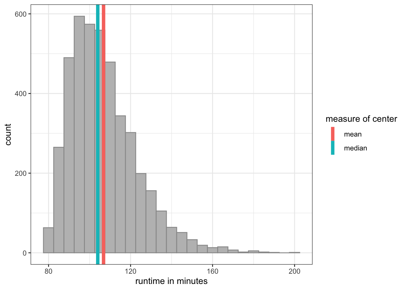
The skew here is not too great, but it pulls the mean almost three minutes higher than the median.
Figure 2.14 shows the distribution of box office returns to movies which is heavily right skewed. Most movies make moderate amounts of money, and then there are a few star performers that make bucket loads of cash.

As a result of this skew, the mean box office returns are about $45.8 million, while the median box office returns are about $18.9 million. The mean here is more than double the median!
Note that neither estimate is in some fundamental way incorrect. They are both correctly estimating what they were intended to estimate. It is up to us to understand and interpret these numbers correctly and to understand their limitations.
Percentiles and the Five Number Summary
In this section, we will learn about the concept of percentiles. Percentiles will allow us to calculate a five number summary of a distribution and introduce a new kind of graph for describing a distribution called the boxplot.
Percentile
We have already seen one example of a percentile. The median is the 50th percentile of the distribution. It is the point at which 50% of the observations are lower and 50% are higher. We can use this exact same logic to calculate other percentiles. We could calculate the 25th percentile of the distribution by finding the point where 25% of the observations are below and 75% are above. We could even calculate the 42nd percentile if we were so inclined.
We calculate percentiles in a fashion similar to the median. First, sort the data from lowest to highest. Then, find the exact observation where X% of the observations fall below to find the Xth percentile. In some cases, there might not be an exact observation that fits this description and so you may have to take the mean across the two closest numbers.
The quantile command in R will calculate percentiles for us in this fashion (quantile is a synonym for percentile). In addition to telling the quantile command which variable we want the percentiles of, we need to tell it which percentiles we want. In the command below, I ask for the 27th and 57th percentile of age in our sexual frequency data.
quantile(sex$age, p=c(.27,.57))27% 57%
36 54 27% of the sample were younger than 36 years of age and 57% of the sample were younger than 54 years of age.
What is the
c() command?
You will notice that for the second argument of quantile I fed in c(.27,.57). What does the c stand for here? It stands for the word concatenate in this case. This command allows us to feed in a bunch of numbers (or words and other things) and combine them together into a vector. You can think of this vector as just a list of numbers. In this case, I used it to feed in two different percentile values I wanted. If I wanted the 25th, 50th, and 75th percentiles instead, I would have used c(.25, .5, .75). We won’t have to use c() very much in the course, but it is a handy R command to know.
The five number summary
We can split our distribution into quarters by calculating the minimum (0th percentile), the 25th percentile, the 50th percentile (the median), the 75th percentile, and the maximum (100th percentile). Collectively, these percentiles are known at the quartiles of the distribution (not to be confused with quantile) and are also described as the five number summary of the distribution.
We can calculate these quartiles with the quantile command. If I don’t enter in specific percentiles, the quantile command will give me the quartiles by default:
quantile(sex$age) 0% 25% 50% 75% 100%
18 35 50 64 89 The bottom 25% of respondents are between the ages of 18-35. The next 25% are between the ages of 35-50. The next 25% are between the ages of 50-64. The top 25% are between the ages of 64-89.
We can also use this five number summary to calculate the interquartile range (IQR) which is just the difference between the 25th and 75th percentile. This gives us a sense of how spread out observations are. In this data:
\[IQR=64-35=29\]
So, the 25th and 75th percentile of age are separated by 29 years.
Boxplots
We can also use this five number summary to create another graphical representation of the distribution called the boxplot. Figure 2.15 below shows a boxplot for the age variable from the sexual frequency data.
1ggplot(sex, aes(x="", y=age))+
2  geom_boxplot(fill="skyblue", outlier.color = "red")+
  labs(x=NULL)+
theme_bw()- 1
-
We use the
yaesthetic to indicate the variable we want the boxplot for. The only unusual thing here is the use ofx=""which we do to avoid having non-intuitive numbers plotted on the x-axis. - 2
-
The
geom_boxplotcommand will graph the boxplot. I have specified a few colors, but these are not necessary. This graph does not have any outliers but setting theoutlier.colorwill help them stand out more in the figure.

The “box” in the boxplot is drawn from the 25th to the 75th percentile. The height of this box is equal to the interquartile range. The median is drawn as a thick bar within the box. Finally, “whiskers” are then drawn to the minimum and maximum of the data. Sometimes, the whiskers are drawn to less than the minimum and maximum if these values are very extreme and instead the whiskers are drawn out to 1.5xIQR in length and then individual points are plotted. In this case there were no extreme values, so the whiskers were drawn all the way out to the actual maximum and minimum.
The boxplot provides many pieces of information. It shows the center of the distribution as measured by the median. It also gives a sense of the spread of the distribution and extreme values by the height of the box and whiskers. It can also show skewness in the distribution depending on where the median is drawn within the box and the size of the whiskers. If the median is in the center of the box, then that indicates a symmetric distribution. If the median is towards the bottom of the box, then the distribution is right-skewed. If the median is towards the top of the box, then the distribution is left-skewed.
The exercise below allows you to adjust a slider to see different percentiles on both a histogram and a boxplot.
In general, boxplots for a single variable do not contain as much information as a histogram and so are generally inferior for understanding the full shape of the distribution. They can be useful for detecting outliers, but the real advantage of boxplots will come in the next chapter when we learn to use comparative boxplots to make comparisons of the distribution of a quantitative variable across different categories of a categorical variable.
Measuring the Spread of a Distribution
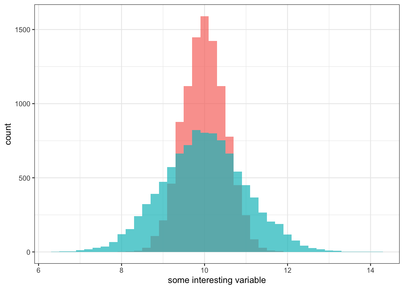
The second most important measure of a distribution is its spread. Spread indicates how far individual values tend to fall from the center of the distribution. As Figure 2.16 below shows, two distributions can have the same center and general shape (in this case, a bell curve) but have very different spreads.
Range and interquartile range
One of the simplest measures of spread is the range. The range is the distance between the highest and lowest value. Lets take a look at the range in the fare paid (in British pounds) for tickets on the Titanic. The summary command, will give us the information we need:
summary(titanic$fare) Min. 1st Qu. Median Mean 3rd Qu. Max.
0.000 7.896 14.454 33.276 31.275 512.329 Note that at least one person made it on the Titanic for free. The highest fare paid was 512.3 pounds. So the range is easy to calculate 512.3 - 0 = 512.3. The difference between the highest and lowest paying passenger was about 512 pounds.
This example also reveals the shortcoming of the range as a measure of spread. If there are any outliers in the data, they will by definition show up in the range and so the range may give you a misleading idea of how spread out the values are. Note that the 75th percentile here is only 31.28 pounds, which would suggest that the 512.3 maximum is a pretty big outlier. We can check this by graphing a boxplot, as I have done in Figure 2.17.
ggplot(titanic, aes(x="", y=fare))+
  geom_boxplot(fill="seagreen", outlier.color = "red")+
  labs(x=NULL, y="fare paid in British pounds")+
  theme_bw()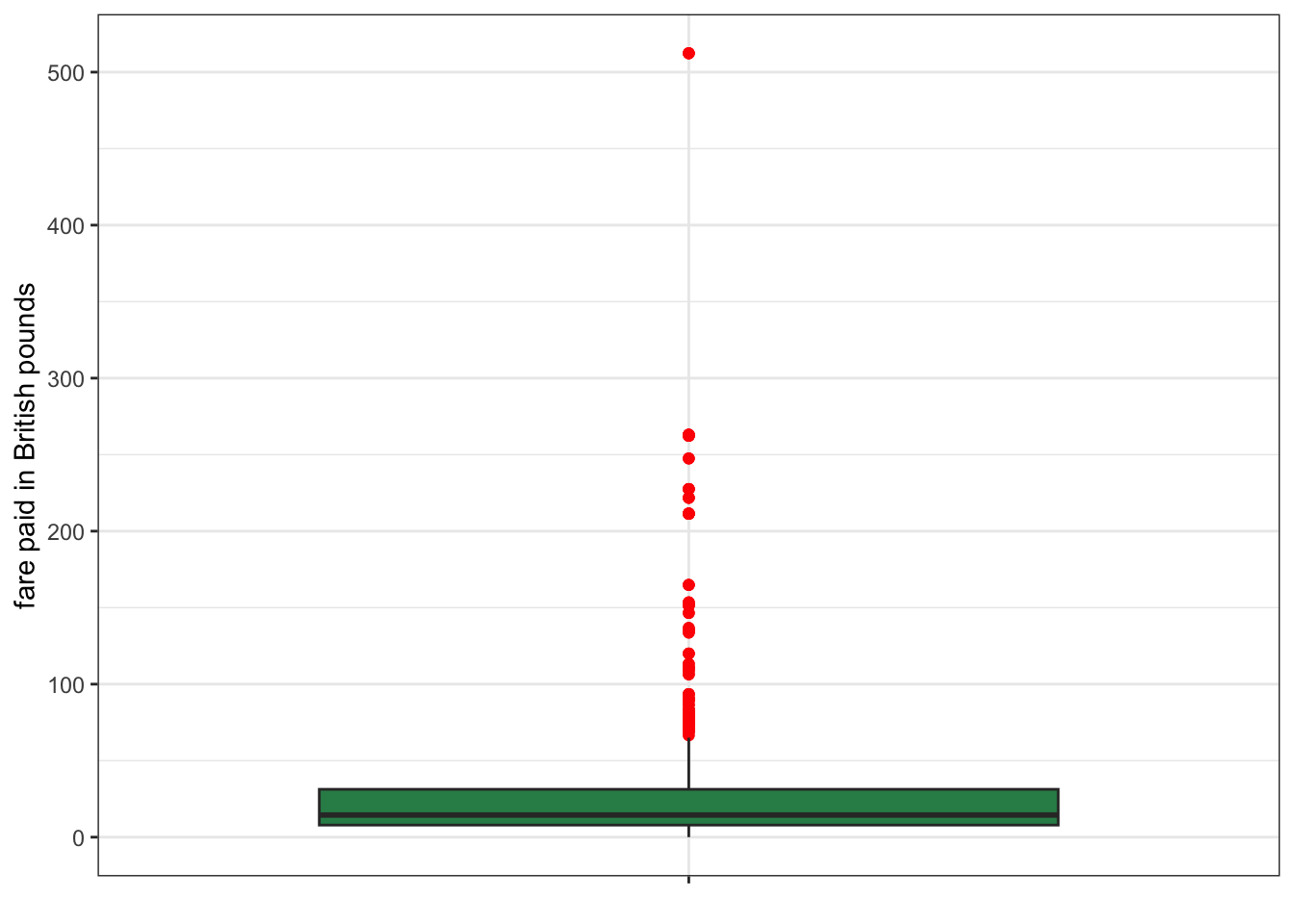
The maximum value is such an outlier that the rest of the boxplot has to be “scrunched” in order to fit it all into the graph. Clearly this is not a good indicator of spread. However, we have already seen a better measure of spread using a similar idea: the interquartile range or IQR. The IQR is simply the range between the 25th and 75th percentile. We already have these numbers from the output above, so the IQR = 31.28-7.90=23.38. The difference in fare between the 25th and 75th percentile (the middle 50% of the data) was 23.4 pounds. That result suggests a much smaller spread of fares for the middle of the distribution.
You can also use the IQR command in R to directly calculate the IQR.
IQR(titanic$fare)[1] 23.3792Variance and standard deviation
The most common measure of spread is the variance and its derivative measurement, the standard deviation. It is so common in fact, that most people simply refer to the concept of “spread” as “variance.” The variance can be defined as the average squared distance to the mean. Of course, “squared distance” is a bit hard to think about, so we more commonly take the square root of the variance to get the standard deviation which gives us the average distance to the mean. Imagine if you were to randomly pick one observation from your dataset and guess how far it was from the mean. Your best guess would be the standard deviation.
The calculation for the variance and standard deviation is a bit intimidating but I will break it down into steps to show it is not that hard. At the same time, I will show you to calculate the parts in R using the fare variable from the Titanic data.
The overall formula for the variance (which is represented as \(s^2\)) is:
\[s^2=\frac{\sum_{i=1}^n (x_i-\bar{x})^2}{n-1}\]
That looks tough, but lets break it down. The first step is this:
\[(x_i-\bar{x})\]
You take each value of your variable \(x\) and subtract the mean from it. This can be done in R easily:
diffx <- titanic$fare-mean(titanic$fare)This measure gives us a description of how far each observation is from the mean which is already kind of a measure of spread, but we can’t do much with it yet because some differences are positive (higher than the mean) and some are negative (lower than the mean). In fact, if we take the mean of these differences, it will be zero by definition because the mean is the balancing point of the distribution.
round(mean(diffx),5)[1] 0The next step is to square those differences:
\[(x_i-\bar{x})^2\]
By squaring the differences, we get rid of the negative/positive problem, because the squared values will all be positive.
diffx.squared <- diffx^2The next step is:
\[\sum_{i=1}^n (x_i-\bar{x})^2\]
We need to sum up all of our values. This sum is sometimes called the sum of squared X or SSX for short. It is already pretty close to a measure of variance already.
ssx <- sum(diffx.squared)The more spread out the values are around the mean, the larger this value will be. However, it also gets larger when we have more observations because we are just taking a sum. To get a number that is comparable across different number of observations, we need to do the final step:
\[s^2=\frac{\sum_{i=1}^n (x_i-\bar{x})^2}{n-1}\]
We are going to divide our SSX value by the number of observations minus one. The “minus one” thing is a bit tricky and I won’t go into the details of why we do it here. When \(n\) is large, this will have little effect and basically you are taking an average of the squared distance from the mean.
variance <- ssx/(length(diffx)-1)
variance
[1] 2677.409So the average squared distance from the mean fare is 2677.409 pounds squared. Of course, this isn’t a very interpretable number, so its probably better to square root it and get the standard deviation:
sqrt(variance)[1] 51.74369So, the average distance from the mean fare is 51.74 pounds.
Note that I could have used the power of R to do this entire calculation in one line:
sqrt(sum((titanic$fare-mean(titanic$fare))^2)/(length(titanic$fare)-1))[1] 51.74369Alternatively, I could have just used the sd command to have R do all the heavy lifting:
sd(titanic$fare)[1] 51.74369